Weak solutions to dirichlet boundary problems
For the final project in Analysis I, my professor asked us to write a paper on a topic adjacent to analysis. Being an applied mathematician, he recommended I study a very specific inequality called Gårding’s inequality.
If you would like to learn more about Gårding’s inequality itself, my paper has all the details about it, the prerequisites to understand it, and an application. In fact, most of the paper covers the necessary material needed to understand what the inequality is even saying (PDE analysis seems to be a lot less abstract than other fields, considering all the machinery I needed). However, for a blog post, I don’t want to bog down any actual interesting results by trying to describe how this inequality functions. This will only focus on the broader subject of weak solutions to PDEs.
What is a Dirichlet boundary problem?
The following is a general formulation of a Dirichlet boundary problem: Given (1) a function on a region $\Omega$ and (2) a function that tells us exactly what the boundary of the region $\partial\Omega$ looks like, can figure out a function $u$, whose partial derivative satisfies both (1) and (2)?
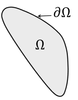
Figure 1. Boundary of a region $\Omega$.
In applied differential equations (physics), Dirichlet boundary problems often show up. If we look at a system that is modeled with differential equations, such as heat flow, fluids, or electricity, and a known boundary, chances are we can derive a Dirichlet boundary problem from it.
Restricting conditions
We will look at a stronger version of this by supposing that the values at the boundary are all zero. With this restriction, there are some useful classifications we have for what a “solution” needs. Let’s assume that we are differentiating $2k$ times (in fact, for Gårding’s inequality to work, the differential operator needs to be elliptic, which requires this condition).
Definition (Classical solution). A function $u$ is a classical solution to the Dirichlet boundary problem if $u$ satisfies the given conditions and is $2k$ times differentiable.
This may seem like the only reasonable way to define a solution, hence the word classical. However, differential equations are extremely hard (you’ll get a million dollars for finding a reasonable solution to the Navier-Stokes equations in $\mathbb{R}^3$), or even impossible to solve. How can we deal with the fact that $u$ may not even exist?
Lifting conditions to define weak solutions
Hence, mathematicians began to come up with the idea of the weak derivative. Weak derivatives allow us to ignore small blips (such as discontinuities) in functions. For example, in calculus you may have shown that the function $f(x)=|x|$ is not differentiable at $x=0$ because the left and right derivatives do not agree. However, our issue is onlys one single point in the whole real number line. So we can create a proxy function that gives the derivative perfectly for almost every point and gives a reasonable value for all the other points. In our case, the following function $v$ works as a weak derivative of $u$: $$ v(t) = \begin{cases} -1 &\text{if }t < 0, \\ 0 &\text{if }t = 0, \\ 1 &\text{if }t > 0. \end{cases} $$ Formalizing this requires the use of integration by parts. We essentially force $v$ to be integrable instead of differentiable in this case, which is a lighter restriction.
Definition (Strong/weak solution). A function $u$ is a strong/weak solution to the dirichlet boundary problem if $u$ is $\approx 2k$ times weakly differentiable.
The “$\approx$” is doing a lot of lifting here by letting me avoid exactly how many times $u$ has to be weakly differentiable. I’m also not specifically distinguishing the strong and weak solutions.
Why does this matter? Well, we can show that all classical solutions are strong solutions, and all strong solutions are weak solutions. However, the other way around is not necessarily true. In theory, there may be weak solutions that are attainable, even if we cannot find any classical ones, and that means we are working with a “larger” class of solutions.
Conclusion
This is my first time working with PDEs past my Calculus III class, and it all was very daunting. However, I noticed it has more immediate applications to the real world via physics. I haven’t covered the linear algebra (norms, inner products, bilinear forms) or higher-level analysis (Lebesgue integration and $L^p$ space) needed to get the full picture, but this does summarize the general idea: lighten conditions to only what you care about when a problem gets very hard.
Perhaps you’re working on a hard exercise and decide to change a restriction: fix a value, go from 3D to 2D, or anything else, and manage to get a solution. There is always a chance that your “weak” solution may helpfully carry over to the “classical” one, or at the very least, can give you insight to solving the problem. :)